Molecular Visualization
All of the structures are represented using JSMol, a free javascript molecular visualizer. Each atom in a strucutre has a unique position given by (x,y,z) coordinates, and a diameter given by a value measured in Angstroms (Å). Each atom is assumed to be a sphere with a defined center and diameter. This simplification drives the visualization and simplifies calculation. Colors are used to show different atom types, the most common being grey for Carbon, white for Hydrogen, red for Oxygen, blue for Nitrogen. MOFs are often crystalline or lattice structures consisting of many repeating units. The smallest such unit is the unit cell and is the default view when a structure is loaded. A supercell arises when a unit cell is repeated several times. To visualize a supercell, imagine that the structure continues from any boundary back around to that accross from it. Or open MOF Explorer and set the supercell parameters.
Periodic Boundary Conditions
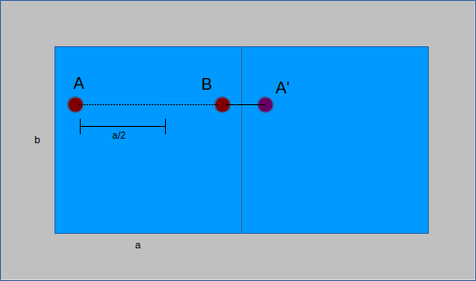
When performing calculations it is often important to know the distance between two structure atoms. Due to periodic boundary conditions (PBC), the nearest atom to a point might not be in the same unit cell. To account for this, all distances are computed twice, as a straight line between points and then taking PBC into consideration. The former yields a distance vector between two points, the latter applies PBC to the vector by considering the image of a point - its analog in the neighboring cell. An important distinction can be made between unit cells that are orthorhombic (all angles are right angles) or not. For those that are, PBC calculations take two steps. First, each component of the distance vector is compared to the unit cell length. If point A is less than half a unit cell from point B, then the image of A in the neighboring cell (A') must be further away. No calculations are made because the original value is the smallest distance. Conversely, if A is more than half the unit cell from B, then A' is closer than A. The distance of A to B becomes the distance from A' to B by shifting the position of A to A':
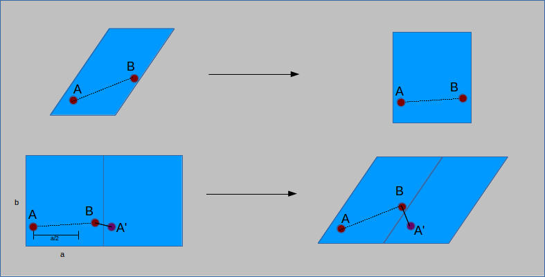
If the cell is not orthorhombic, some of the implicit simplifications above no longer hold. Instead, matrix transformations are used to compute the distance to the image. There is a matrix
that defines any unit cell and can be found with:
	// A, B, C are vector lengths

	// (b) is in the xz-plane and (c) has a positive y component.

	// alpha is the angle (bc), beta is (ac), gamma is (ab)

	a_x = A;

	a_y = 0.0;

	a_z = 0.0;

	b_x = B * Math.cos(gamma);

	b_y = B * Math.sin(gamma);

	b_z = 0.0;

	c_x = C * Math.cos(beta);

	c_y = (B * C * Math.cos(alpha) - b_x * c_x) / b_y;

	c_z = Math.sqrt(Math.pow(C,2) - Math.pow(c_x,2) - Math.pow(c_y,2));


	cellMatrix = [a_x, a_y, a_z, b_x, b_y, b_z, c_x, c_y, c_z];
The inverse of the cell matrix allows for the transformation of the cell to a non-slanted, or orthogonal basis. The same calculations as for an orthorhombic cell are then performed, subtracting
a vector length from the position if the distance is more than half of the vector (here unit cell and vector are not interchangeable). The distance vector is then transformed back to the
original basis by multiplication of the cell matrix. The result is a modified distance vector that takes into account PBC:
To determine if the cell is orthorhombic, a check is performed to see if the cell lengths are all equal and all angles are 90°. Based on the result, PBC are calculated using one of the two above methods.
function pbCond(dist) {


	if (notOrthorhombic) {

		fractional = [0,0,0];

		fractional = matrixDotVector(inverseMatrix, dist);

		xVect = [0,0,0];

		xVect[0] = fractional[0] - Math.round(fractional[0]);

		xVect[1] = fractional[1] - Math.round(fractional[1]);

		xVect[2] = fractional[2] - Math.round(fractional[2]);

		cartesian = matrixDotVector(cellMatrix, xVect);

		return cartesian;

	}


			else {

			if (dist[0] > cellSize[0]/2) {

					dist[0] = dist[0] - cellSize[0];

			}

			if (dist[1] > cellSize[1]/2) {

					dist[1] = dist[1] - cellSize[1];

			}

			if (dist[2] > cellSize[2]/2) {

					dist[2] = dist[2] - cellSize[2];

			}

		return dist;

		}
		}
Void Fraction
The void fraction of a structure is a measure of the volume it occupies within a unit cell. A hollower or emptier cell corresponds to a greater void fraction. Calculating the void fraction is akin to throwing a large number of darts at the structure and seeing how many hit. Instead of darts the simulation uses spherical probes of a given size (point probes have size 0). These probes are inserted randomly into the unit cell and those that overlap with the structure are removed. This is done by comparing the distance from the probe to each of the structure atoms with the sum of their radii. If the sum of the radii is larger than the distance, then the two overlap and the probe is flagged for deletion.
The ratio of those that remain to the total used is the void fraction.
	for (i=0;i<numProbes;i++) { // for all of the probes


		x1 = probeLocation[i][0];

		y1 = probeLocation[i][1];

		z1 = probeLocation[i][2];


		var dr = 0;

		for (k=0;k<numStructureAtoms;k++) { // compare to coordinates of structure


			if (!isInArray(i,flagged)) {

			x2 = atomLocation[k]['x'];

			y2 = atomLocation[k]['y'];

			z2 = atomLocation[k]['z'];


			radius = atomDiameters[atoms[k]['sym']]/2;


			dist = distance(x1,y1,z1,x2,y2,z2);


			dist = pbCond(dist);


			dr = Math.sqrt(Math.pow(dist[0],2) + Math.pow(dist[1],2) + Math.pow(dist[2],2));


			if (dr > (probeRadius + radius)) {

				flagged[index] = i;

				index++;

			} 	}  }  }

			flaggedProbeCount = flagged.length;

			vFraction = 1-flaggedProbeCount/numProbes;
This calculation makes use of a function pbCond which accepts the distance vector between two points as an argument and returns a distance vector. Details of periodic boundary
conditions can be found above in the periodic boundary conditions section.
Surface Area
The surface area of a MOF is a measure of the exposure of atoms to their surroundings. The term surface area conventionally refers to the van der Waals surface area which can be thought of as the size of a sheet required to cover a structure. Another measure of surface area is the solvent-accessible surface area which considers only the surfaces where a solvent molecule could be found.
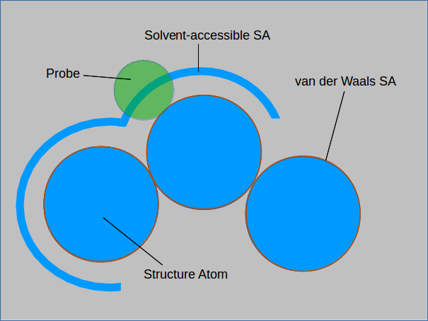
The absolute and solvent-accessible surface areas are equivalent for a solvent of size 0. Measuring the solvent-accessible surface area can be thought of as rolling
a ball over the entire surface and measuring the area covered. Larger spheres will not be able to enter cavities in the structure and will result in a smaller measured surface area.
The surface area is measured by first randomly placing probes on the surface of structure atoms. This is achieved by taking the center of a structure atom and genrating random points
at a fixed distance from it. The distance is the sum of the radii of the structure atom and the probe. The following code shows how to generate uniformly distributed points on the surface of
a sphere:
	theta = 2*Math.PI*Math.random();

	phi = Math.acos(2*Math.random()-1.0);

	xu = Math.cos(theta)*Math.sin(phi);

	yu = Math.sin(theta)*Math.sin(phi);

	zu = Math.cos(phi);


	rad = atomRad + probeRad;


// x, y, z are the location of the structure atom in question


	probeX = x + rad*xu;

	probeY = y + rad*yu;

	probeZ = z + rad*zu;
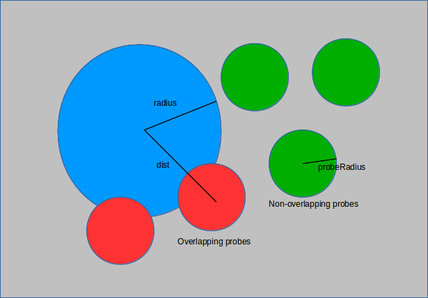
A check is perfomed to see if the probe overlaps with any other structure atoms (with PBC considered). If it does not, a counter is incremented to indicate a successfully placed probe. Once the atom is done being probed, its accessible surface area is computed.
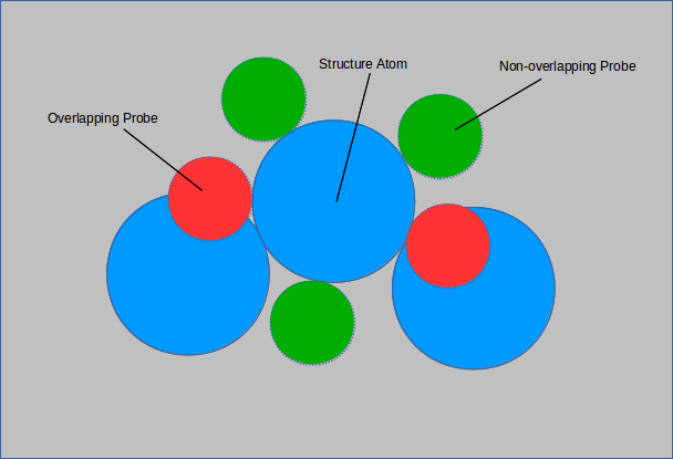
In the above figure, 3 out 5 of the probes do not overlap with any structure atoms. The surface area of the structure atom in question
is (3/5 π r 2).
	for (i=0;i<probesPerAtom;i++) { // for each of the probes given per atom

		overlapP = probeOverlap([probeX,probeY,probeZ]);

if (!overlapP) { // if probe has no overlaps

		notOverlap++; // increment number of non-overlapped

	}


	if (i == probesPerAtom -1) { // on the last iteration of the for loop, compute the surface area

		totalRad = atomRad + probeRad; // sum of radii

		// surface area of sphere S with radius (r(probe) + r(atom)) * non-overlapping probe fraction

		surfaceArea = 4*Math.PI*Math.pow(totalRad,2)*notOverlap/probesPerAtom;

		}
	}
This is repeated for all of the structure atoms and the resultant volumetric and gravimetric surface areas (using atomic masses) are given.
Pore Size Distribution
Some MOFs are finding applications for gas adsorption due to their highly porous nature. The pores of a MOF can be quantified using a pore size distribution (PSD). The PSD is a measure
of the size and relative availability of pores in a structure and is presented as a plot of pore size and relative abundance. Finding the size of a pore using random sampling requires
locating the largest sphere that encompasses a given point but does not overlap with any of the structure atoms.
The PSD is the only physical property here that is not measured using a Monte Carlo simulation. Instead a more optimal algorithm is employed.
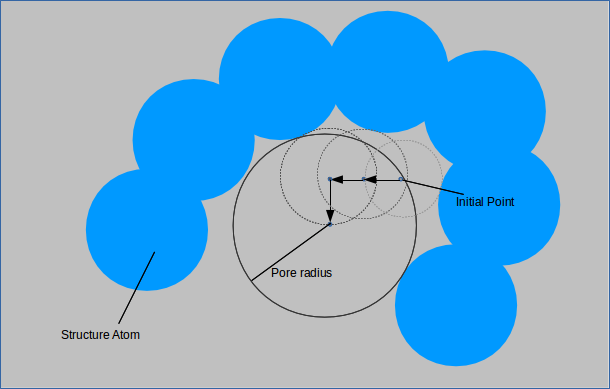
For each of the probes specified a random point is generated outside of any structure atoms. A small sphere is made centered at this point and its radius incremented until it overlaps with a structure
atom. The point is then moved slighlty in each of the six directions and the procedure is repeated. If a larger sphere can be made centered at a shifted point and this sphere encompasses the
original point, then it is accepted as the new standard against which spheres are compared when this procedure is repeated. When shifting the point slightly no longer yields a larger sphere,
the largest probe size is recorded as the pore size for that point. This is performed with points uniformly distributed throghout the unit cell gives the pore size distribution which is normalized
and plotted.
 for (q=0;q<numProbes;q++) {


	r = largestRadius(probePoint,0); // find the largest radius at the point, beginning with 0

	testPointArray = incrementPoint(probePoint); // create an array of points shifted from the original point slightly


	// recursively find the largest pore by finding the largest radius at each of the shifted points

	// take the point which yields the largest radius, create an array of shifted points from there and repeat

	probeSize = findPore(testPointArray,r);


	probeSizeArray = binArray(probeSize,probeSizeArray); // for graphing purposes bin the array of pore sizes to the probe size found - the negative derrivative of this array is plotted

}


function largestRadius(point,startingRadius) {

	i=startingRadius;

	while (!checkOverlap(point,i)) {

		i+=stepSize;

	}

	return i;

}


function incrementPoint(point) { // six directions, + x,y,z; - x,y,z

	pointArray = [];

	for (j=0;j<3;j++) {

		up[j] = point[j] + step; // step is a fixed stepsize of 0.05

		down[j] = point[j] - step;

	}

	pointArray[0] = [up[0], point[1], point[2]];

	pointArray[1] = [point[0], up[1], point[2]];

	pointArray[2] = [point[0], point[1], up[2]];

	pointArray[3] = [down[0], point[1], point[2]];

	pointArray[4] = [point[0], down[1], point[2]];

	pointArray[5] = [point[0], point[1], down[2]];


	return pointArray;

}
Plotting is performed with a javascript library called flot.